
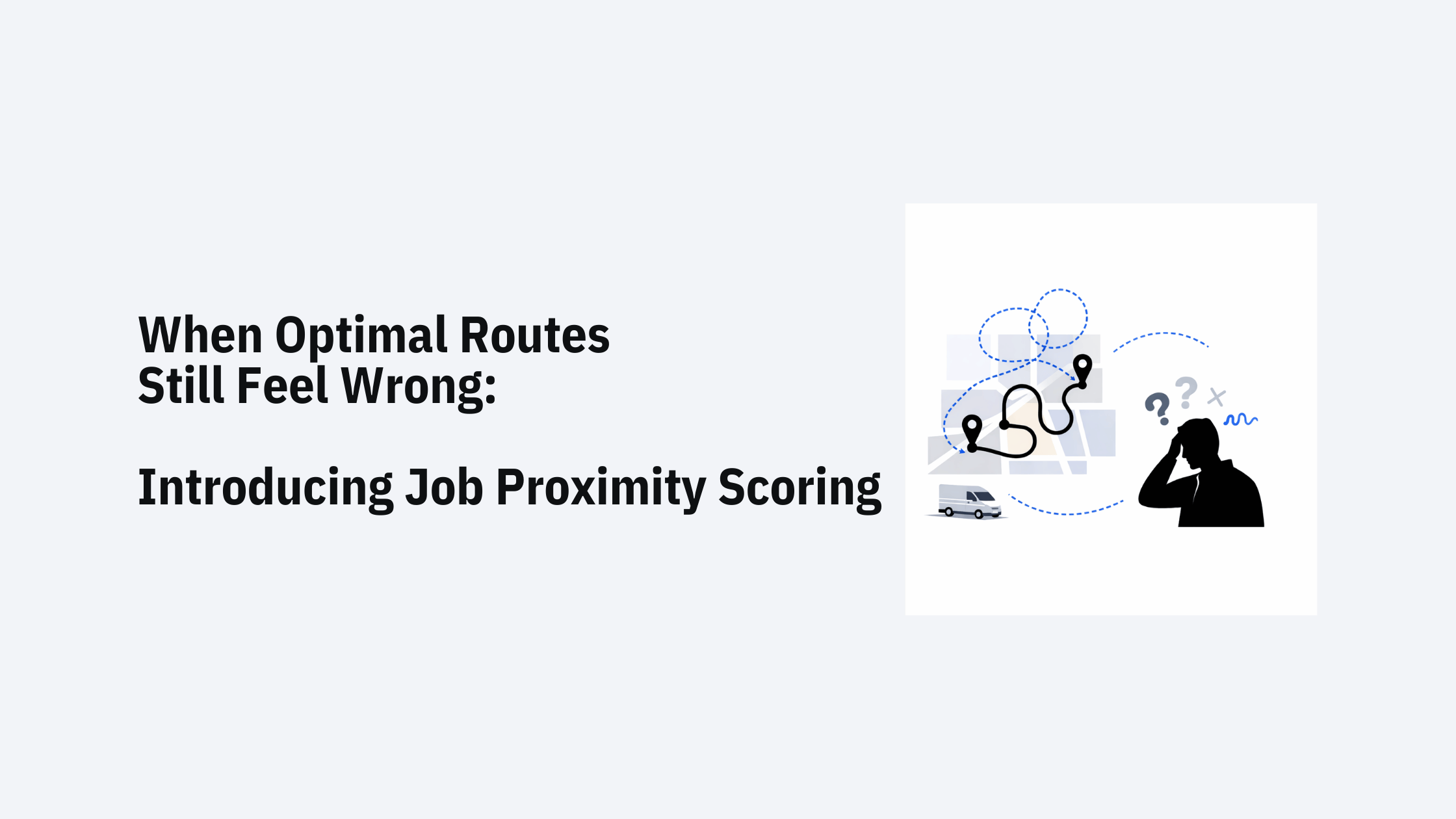
Mathematically optimal routes can still frustrate drivers. Your route optimizer minimizes total travel time, but your courier gets sent back to the same street three times in one shift. The system says it's efficient. Your driver disagrees.
This disconnect between algorithmic optimization and practical routing surfaces regularly in last-mile delivery. Even when travel time is minimized, routes that revisit the same geographic area multiple times create unnecessary complexity. Drivers make wrong turns returning to neighborhoods they just left. GPS systems recalculate repeatedly. What looks efficient on paper feels wasteful on the ground.
Traditional route optimization algorithms focus on minimizing total distance or time. They're good at this—VRP solvers have decades of research behind them. But they treat every job as an independent point in space, optimizing the sequence without considering geographic clustering.
The result: a route might send a technician to job A in neighborhood 1, then to job B in neighborhood 2, then back to job C in neighborhood 1—because that sequence minimizes the total route time by 3 minutes compared to completing A and C consecutively.
Most routing systems address this through rigid pre-grouping. Planners manually cluster jobs into geographic zones before optimization begins, or the system automatically merges nearby jobs into compound stops. Both approaches sacrifice flexibility. Pre-grouped jobs can't be reassigned across zones when time windows conflict or vehicle capacity is exceeded. Merged stops become inflexible units that prevent granular optimization.
Solvice's Job Proximity Scoring treats geographic clustering as an optimization signal rather than a hard boundary. Instead of forcing jobs into predefined groups, the feature encourages the optimizer to complete nearby jobs consecutively—while still allowing the algorithm to break this preference when other constraints demand it.
The mechanic is straightforward: you define a proximity radius (between 50m and 1500m) around each job. When the optimizer considers completing two jobs back-to-back within this radius, it receives a positive score. When it routes a vehicle away from a cluster before completing all nearby jobs, it incurs a penalty.
The strength of this preference is controlled by a weight parameter. Set it too low, and the optimizer ignores proximity entirely. Set it too high, and you recreate the rigidity of pre-grouped zones. The optimal setting depends on your specific operation—high-density urban delivery needs tighter clustering than rural service routes.
The feature operates during route optimization, not as a preprocessing step. As the metaheuristic explores different route sequences, proximity scoring influences which solutions score higher in the objective function.
When evaluating a route sequence, the optimizer calculates:
The algorithm continues to optimize across all constraints simultaneously. A route might still split a cluster if doing so prevents a time window violation or balances vehicle capacities more effectively. Proximity is a preference, not a requirement.
Job Proximity Scoring requires two configuration values:
Proximity Radius (50m - 1500m): Defines the geographic range for clustering jobs. Common settings:
Proximity Weight: Controls how strongly the optimizer should favor geographic clustering relative to other objectives. Start with moderate values and adjust based on route acceptance rates and driver feedback.
The feature works with all standard VRP constraints. Jobs with time windows, capacity requirements, or skill matching still respect those constraints—proximity scoring simply adds another factor to the optimization objective.
An e-commerce delivery service operates in a downtown area with 200+ delivery points per day clustered in commercial districts. The optimizer tends to fragment routes across neighborhoods when optimizing purely for time.
Setting a 200m proximity radius encourages street-by-street completion. The courier clears an entire block before moving to the next street, reducing navigation errors and missed addresses. The GPS system stops recalculating as frequently because the courier isn't zigzagging across the service area.
A maintenance contractor services office buildings across several business parks. Each park contains 5-15 buildings spread across 500-800m. Without proximity clustering, technicians might visit Park A in the morning, drive to Park B, then return to Park A in the afternoon—because the afternoon job has a 2-4 PM time window and the algorithm optimized around that constraint.
A 600m proximity radius with moderate weighting helps the optimizer recognize when it's worth extending a morning time window slightly to keep all Park A jobs in one visit. The technician completes the park in one trip rather than returning later, reducing total vehicle miles even if it means arriving at one job 15 minutes earlier than optimal.
This feature targets operations where:
It's less useful for:
Job Proximity Scoring adds another dimension to the multi-objective optimization problem that VRP solvers already manage. The algorithm balances:
You control the relative importance through weight parameters. In practice, start with moderate proximity weights and monitor:
The optimal balance depends on your operation's priorities. High-density operations with tight time windows might use lighter proximity weights. Lower-density service routes with flexible scheduling might weigh proximity more heavily.
Job Proximity Scoring is configured per optimization request through the Solvice API. No preprocessing or manual grouping is required—you specify the radius and weight, and the optimizer handles the rest.
The feature works with:
For dynamic scheduling operations, proximity scoring helps maintain route stability. When new jobs arrive mid-route, the optimizer can insert them into existing geographic clusters rather than creating new ones, reducing driver confusion about route changes.
Read the full documentation about Job Proximity Scoring here.
Route optimization algorithms excel at solving complex mathematical problems. But the quality of a route isn't determined solely by minimizing an objective function—it's also defined by driver acceptance, operational efficiency, and customer experience.
Job Proximity Scoring bridges the gap between computational efficiency and practical routing. By treating geographic clustering as an optimization signal rather than a rigid constraint, it helps create routes that feel intuitive to drivers while maintaining the flexibility needed for complex scheduling operations.
The feature is available now in the Solvice OnRoute VRP API. Start with a moderate proximity radius (200-400m for urban routes, 600-1000m for suburban/rural), set a reasonable weight, and adjust based on actual route performance.
For implementation details and API documentation, see the Job Proximity Scoring guide in the Solvice documentation.


.png)